This page was generated from docs/Examples/Fitting_Water_Silicate_Melts/Example4b_H2OQuant_MI/H2O_Fitting_MI_AutoLoop.ipynb. Interactive online version: .

Python Notebook Download

Fitting H2O and Silicate areas from unexposed MIs (looping)

• This notebook shows how to quantify the relative area of the silicate peak and H2O peak from acquisitions of olivine-hosted melt inclusions still at depth in the crystal. Specifically, the code unmixes the olivine and melt inclusions spectra to obtain the glass spectra

• In this example, we loop through multiple files, as we find we can use the same peak parameters for all of them

• If you want an example where you manually loop through files, see the exapmle ‘H2O_Fitting_MI_ManualLoop’

Import necessary python things

import numpy as np
import pandas as pd
import matplotlib.pyplot as plt
import DiadFit as pf
pf.__version__

'1.0.3'

# This is where you tell the code where your spectra are. E.g. DayFolder is the overal folder, if you have subfolders for Spectra and MetaData
import os
DayFolder=os.getcwd()
meta_path=DayFolder +  '\MetaData'
spectra_path=DayFolder + '\Spectra'
file_ext='.txt'
filetype='Witec_ASCII'

# Get the files which are the melt inclusion/H2O acquisitoin first. You need a unique string (here H2O) which is in all files
MI_Files=pf.get_files(path=spectra_path,
file_ext=file_ext, ID_str='H2O',
exclude_str=['depth', 'line', 'scan'], sort=False)
MI_Files

['02 CC14_MI2_H2O_96mw.txt',
 '05 CC13_MI4_H2O.txt',
 '09 CC9_MI3_H2O.txt',
 '12 CC9_MI1_H2O_20X.txt',
 '15 CC9_MI1_H2O_50X.txt',
 '18 CC5_MI1_H2O_10mw.txt',
 '21 CC7_MI3_H2O.txt',
 '24 CC4_MI1_H2O.txt',
 '29 MS13_2_MI1_H2O.txt']

# These are the files for the acquisition in the neighbouring host mineral - in this case, the unique file string is 'Ol'
Host_Files=pf.get_files(path=spectra_path,
file_ext=file_ext, ID_str='Ol',
exclude_str=['depth', 'line', 'scan'], sort=False)
Host_Files

['03 CC14_MI2_Ol_96mw.txt',
 '06 CC13_MI4_Ol.txt',
 '10 CC9_MI3_Ol.txt',
 '16 CC9_MI1_Ol_50X.txt',
 '19 CC5_MI1_Ol.txt',
 '22 CC7_MI3_Ol.txt',
 '25 CC4_MI1_Ol.txt',
 '30 MS13_2_MI1_Ol.txt']

Now we want to split up the name into its key parts - this will allow us to match a given melt inclusion file to the host olivine file

char_crystal='_' # This is what you separated your string based on, e.g. here we use underscores
print(Host_Files[0].split(char_crystal))

['03 CC14', 'MI2', 'Ol', '96mw.txt']

# Here you define what characters separate MI and crystal names. First, we are looking at the files of our host olivine.
pos_crystal=0 # This is which character is the crystal name, e.g. ignoring the prefix, the crystal in the above example is CC14
pos_MI=1 # This is the unique melt inclusion, in the example above this is MI2, which is the second position in the array (so 1 in python which starts counting at zero)
char_MI='_' # If you split your MI using a different string
Host_Files_extract=pf.extract_xstal_MI_name(files=Host_Files, prefix=True, str_prefix=' ',
char_xstal=char_crystal, pos_xstal=pos_crystal, char_MI=char_MI, pos_MI=pos_MI, file_ext=file_ext)
Host_Files_extract.head()

good job, no duplicate file names

	filename	crystal_name	MI_name
0	03 CC14_MI2_Ol_96mw.txt	CC14	MI2
1	06 CC13_MI4_Ol.txt	CC13	MI4
2	10 CC9_MI3_Ol.txt	CC9	MI3
3	16 CC9_MI1_Ol_50X.txt	CC9	MI1
4	19 CC5_MI1_Ol.txt	CC5	MI1

# Now do the same for your melt inclusion files
print(MI_Files[0].split('_'))

['02 CC14', 'MI2', 'H2O', '96mw.txt']

MI_Files_extract=pf.extract_xstal_MI_name(files=MI_Files,prefix=True, str_prefix=' ',
char_xstal=char_crystal, pos_xstal=pos_crystal, char_MI=char_MI, pos_MI=pos_MI)
MI_Files_extract.head()

good job, no duplicate file names

	filename	crystal_name	MI_name
0	02 CC14_MI2_H2O_96mw.txt	CC14	MI2
1	05 CC13_MI4_H2O.txt	CC13	MI4
2	09 CC9_MI3_H2O.txt	CC9	MI3
3	12 CC9_MI1_H2O_20X.txt	CC9	MI1
4	15 CC9_MI1_H2O_50X.txt	CC9	MI1

# This aligns the H2O and silicate file based on the same value for the column xstal name and MI name
merge=MI_Files_extract.merge(Host_Files_extract, on=['crystal_name', 'MI_name' ], how='inner')
merge.head()

	filename_x	crystal_name	MI_name	filename_y
0	02 CC14_MI2_H2O_96mw.txt	CC14	MI2	03 CC14_MI2_Ol_96mw.txt
1	05 CC13_MI4_H2O.txt	CC13	MI4	06 CC13_MI4_Ol.txt
2	09 CC9_MI3_H2O.txt	CC9	MI3	10 CC9_MI3_Ol.txt
3	12 CC9_MI1_H2O_20X.txt	CC9	MI1	16 CC9_MI1_Ol_50X.txt
4	15 CC9_MI1_H2O_50X.txt	CC9	MI1	16 CC9_MI1_Ol_50X.txt

Select file

• select a file to tweak fit parameters

# Just choose 1 file to have a look
i=0
filename_MI=merge['filename_x'].iloc[i]
filename_Host=merge['filename_y'].iloc[i]
print(merge['filename_y'].iloc[i])

03 CC14_MI2_Ol_96mw.txt

# This pulls out the host file and the MI file
spectra_Host=pf.get_data(path=spectra_path, filename=filename_Host,
            Diad_files=None, filetype=filetype)

spectra_MI=pf.get_data(path=spectra_path, filename=filename_MI,
            Diad_files=None, filetype=filetype)

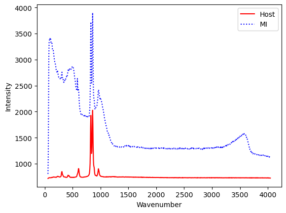
First plot spectra

plt.plot(spectra_Host[:, 0], spectra_Host[:,1], '-r', label='Host')
plt.plot(spectra_MI[:, 0], spectra_MI[:,1], ':b', label='MI')
plt.legend()
plt.xlabel('Wavenumber')
plt.ylabel('Intensity')

Text(0, 0.5, 'Intensity')

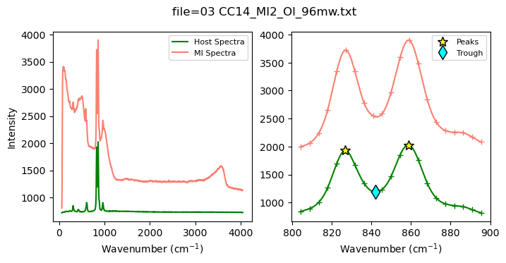
Now, lets smooth and trim the spectra, and find the peaks

x_new, y_cub_MI, y_cub_Host, peak_pos_Host, peak_height_Host, trough_x, trough_y, fig=pf.smooth_and_trim_around_host(
x_range=[800,900], x_max=900, Host_spectra=spectra_Host,
MI_spectra=spectra_MI, filename=filename_Host)
fig.savefig('smooth_Spline.png', dpi=300, bbox_inches='tight')

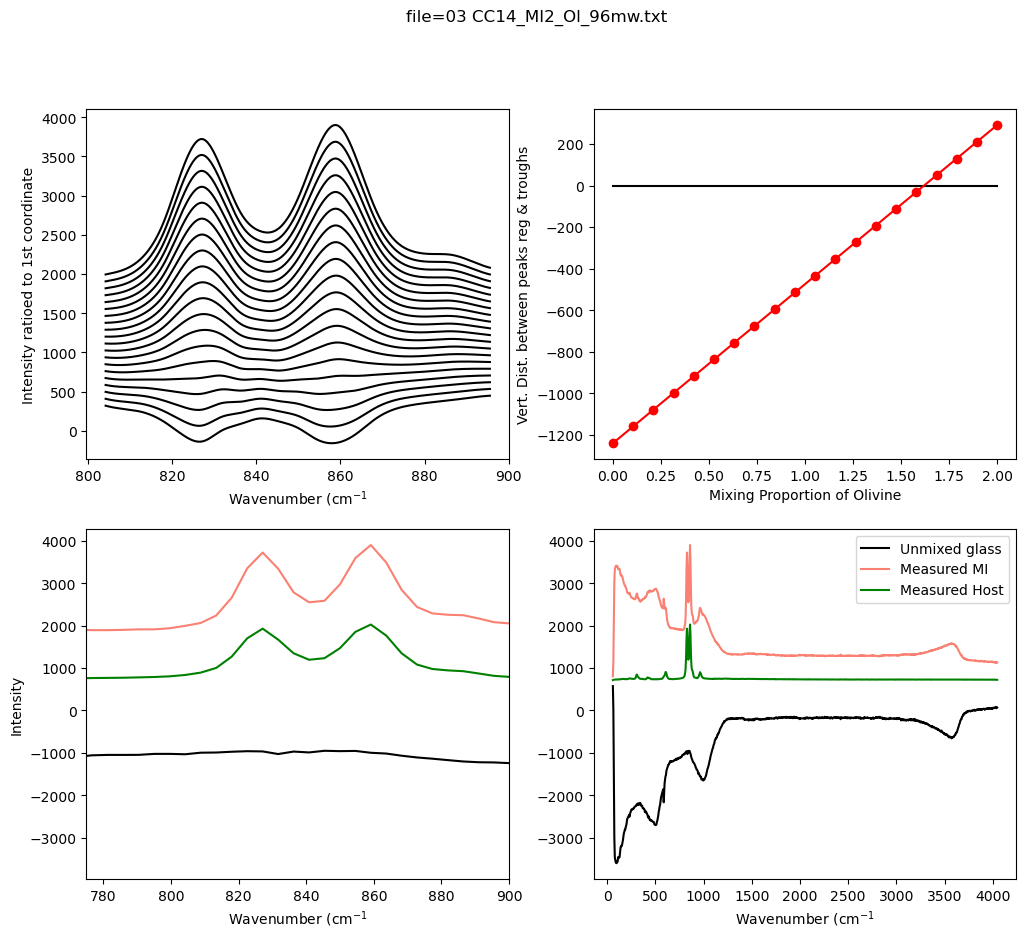
Now lets look at different mixing proportions

MI_Mix_Best, ideal_mix, Dist, MI_Mix, X=pf.make_evaluate_mixed_spectra(
path=spectra_path, filename=filename_Host,
smoothed_host_y=y_cub_Host, smoothed_MI_y=y_cub_MI,
Host_spectra=spectra_Host, MI_spectra=spectra_MI, x_new=x_new,
peak_pos_Host= peak_pos_Host,
trough_x=trough_x, trough_y=trough_y, N_steps=20, av_width=2,
X_min=0, X_max=2)

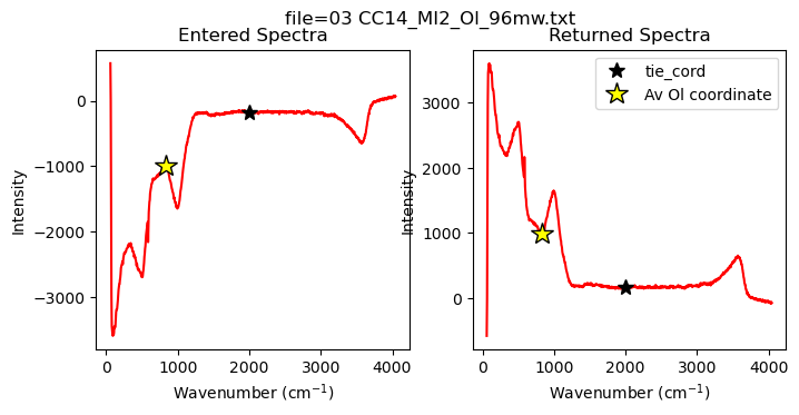
check if spectra needs inverting

• Sometimes the best fit spectra will end up upsideown, this inverts it if this happens

Spectra2=pf.check_if_spectra_negative(Spectra=MI_Mix_Best,
path=spectra_path, filename=filename_Host,
peak_pos_Host=peak_pos_Host, tie_x_cord=2000, override=False, flip=True)

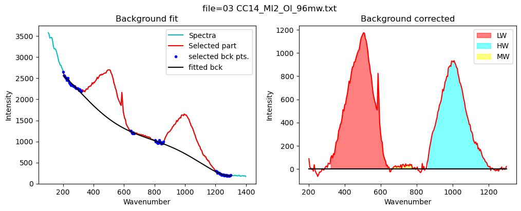
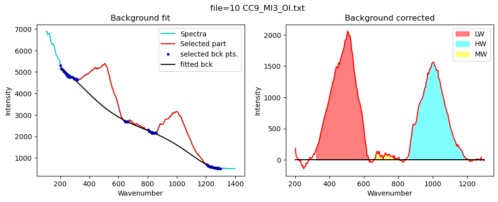
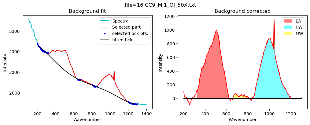
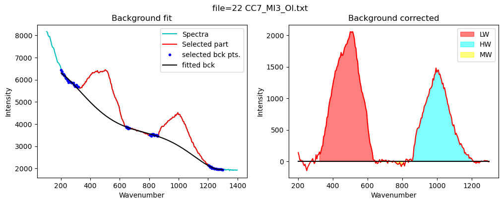
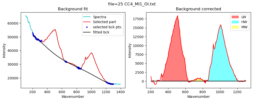
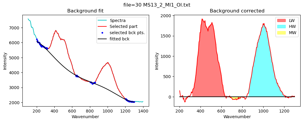
Now lets quantify the area under the silicate region

• Set up the background postiions, can overwrite default

config_silicate=pf.sil_bck_pos_Schiavi_basalt(
lower_range_sil=(200, 320),
mid_range1_sil=(640, 670), mid_range2_sil=(800, 860),
upper_range_sil=(1200, 1300),
N_poly_sil=5)

print(config_silicate)
df_sil=pf.fit_area_for_silicate_region(Spectra=Spectra2,
path=spectra_path, filename=filename_Host, config1=config_silicate,
 plot_figure=True,
fit_sil='poly')
df_sil

sil_bck_pos_Schiavi_basalt(lower_range_sil=(200, 320), mid_range1_sil=(640, 670), mid_range2_sil=(800, 860), upper_range_sil=(1200, 1300), LW=(400, 600), HW=(800, 1200), N_poly_sil=5, sigma_sil=5)

	Silicate_LHS_Back1	Silicate_LHS_Back2	Silicate_RHS_Back1	Silicate_RHS_Back2	Silicate_N_Poly	Silicate_Trapezoid_Area	Silicate_Simpson_Area	LW_Silicate_Trapezoid_Area	LW_Silicate_Simpson_Area	HW_Silicate_Trapezoid_Area	HW_Silicate_Simpson_Area	MW_Silicate_Trapezoid_Area	MW_Silicate_Simpson_Area
0	200	320	1200	1300	5	379864.496263	379745.013178	198303.832398	198693.030414	163488.966895	163563.287063	2856.492903	2889.766264

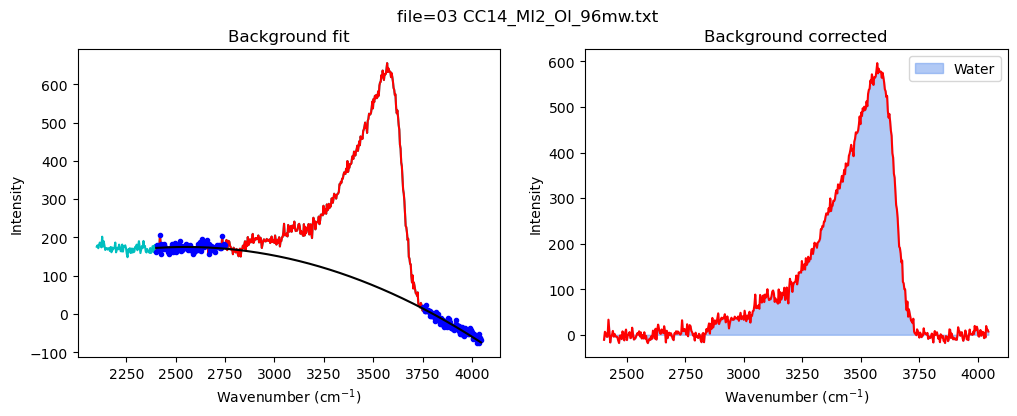
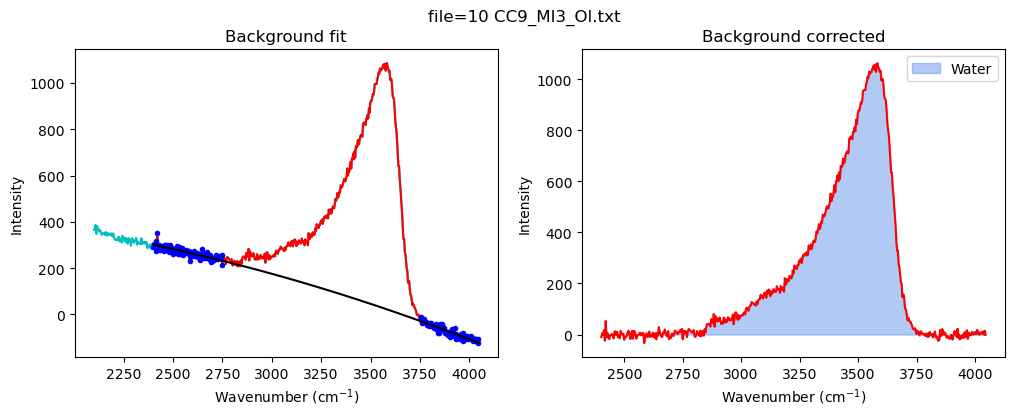
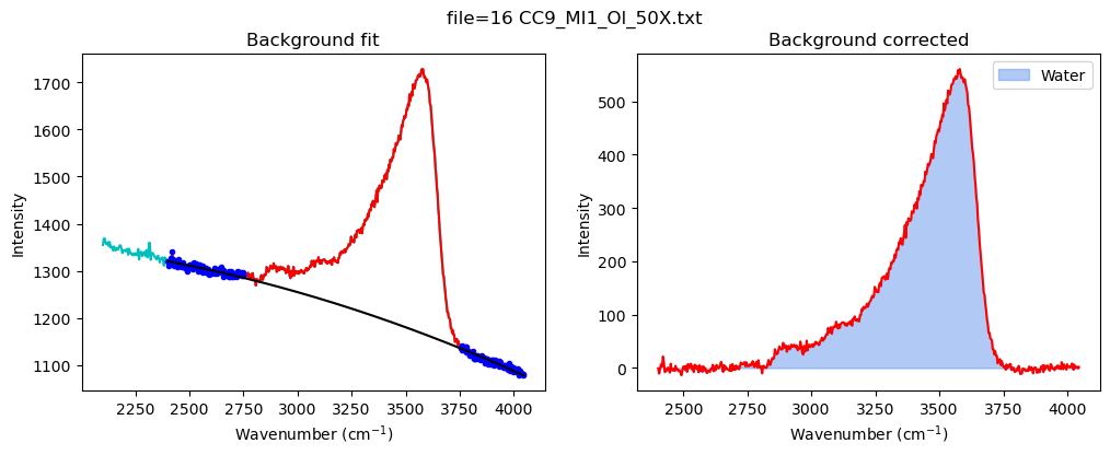
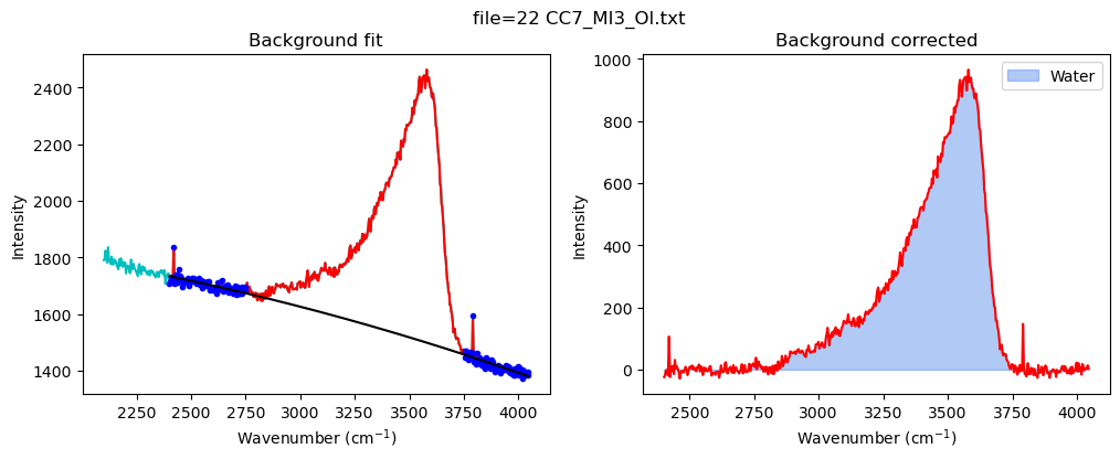
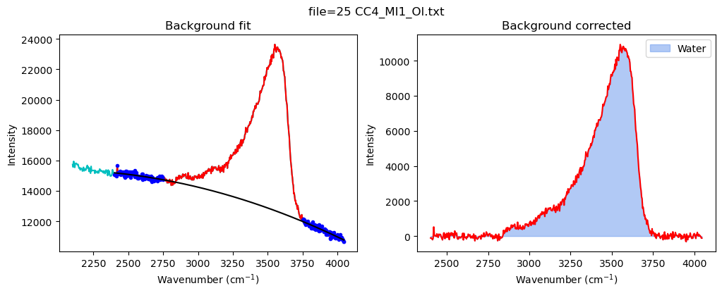
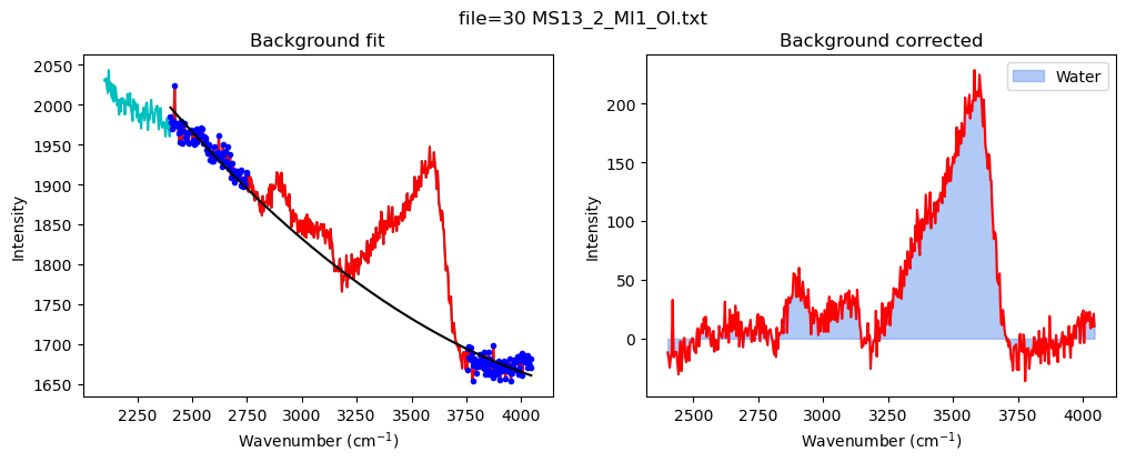
Now quantify the area under the water region

config_MI=pf.water_bck_pos(lower_bck_water=(2400, 2750),
N_poly_water=2)
print(config_MI)
df_MI=pf.fit_area_for_water_region(
path=spectra_path, filename=filename_Host,
Spectra=Spectra2, config1=config_MI, plot_figure=True)

water_bck_pos(fit_water='poly', N_poly_water=2, lower_bck_water=(2400, 2750), upper_bck_water=(3750, 4100))

combo_out=pf.stitch_dataframes_together(df_sil=df_sil, df_water=df_MI,
Host_file=filename_Host, MI_file=filename_MI)
combo_out

	Host filename	MI filename	Water_to_HW_ratio_Trapezoid	Water_to_HW_ratio_Simpson	Water_to_Total_Silicate_ratio_Trapezoid	Water_to_Total_Silicate_ratio_Simpson	Water_Trapezoid_Area	Water_Simpson_Area	Silicate_Trapezoid_Area	Silicate_Simpson_Area	...	HW_Silicate_Trapezoid_Area	HW_Silicate_Simpson_Area	MW_Silicate_Trapezoid_Area	MW_Silicate_Simpson_Area	Water Filename	Water_LHS_Back1	Water_LHS_Back2	Water_RHS_Back1	Water_RHS_Back2	Water_N_Poly
0	03 CC14_MI2_Ol_96mw.txt	02 CC14_MI2_H2O_96mw.txt	1.29263	1.291034	0.556332	0.556073	211330.717146	211165.80878	379864.496263	379745.013178	...	163488.966895	163563.287063	2856.492903	2889.766264	03 CC14_MI2_Ol_96mw.txt	2400	2750	3750	4100	2

1 rows × 27 columns

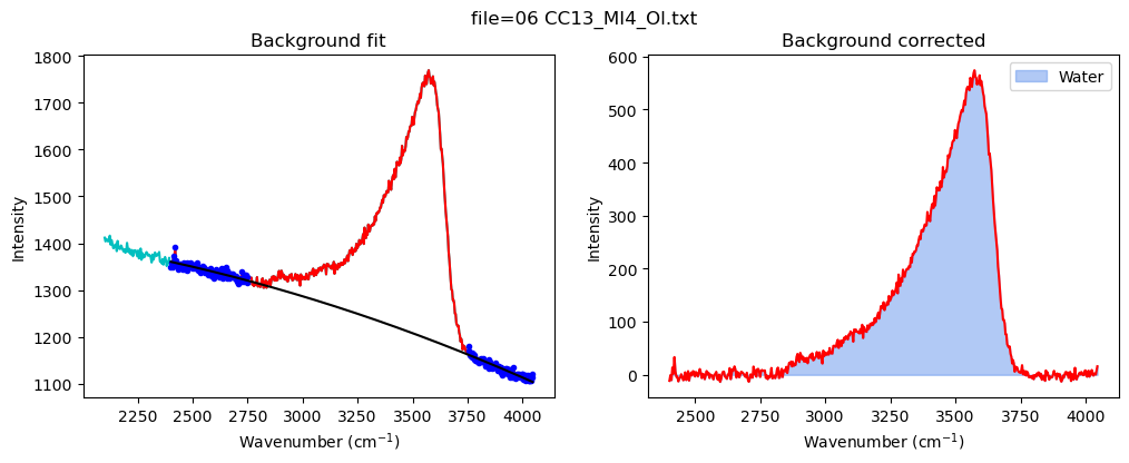
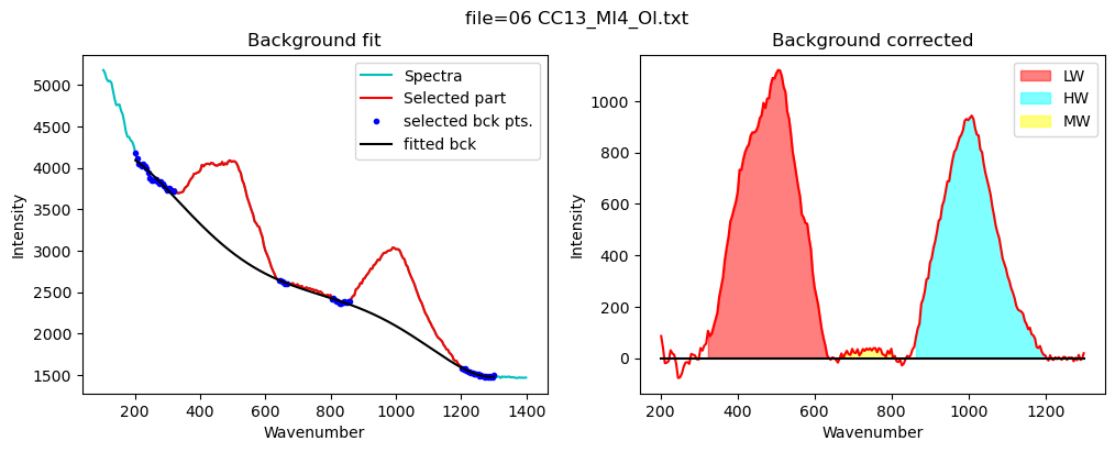
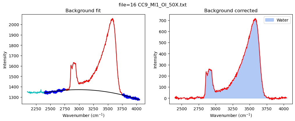
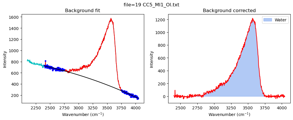
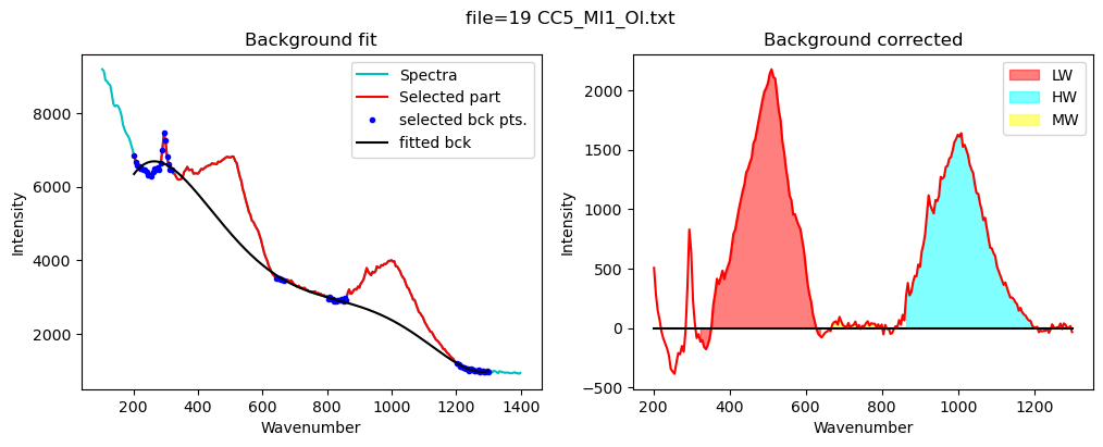
Now we have set it up for one melt inclusion host pair, we can use the same parameters to loop through all files

## Now lets loop through all files
from tqdm import tqdm

df_merged=pd.DataFrame([])
for i in tqdm(range(0, len(merge))):
    filename_MI=merge['filename_x'].iloc[i]
    filename_Host=merge['filename_y'].iloc[i]


    # Get files
    spectra_Host=pf.get_data(path=spectra_path, filename=filename_Host,
            Diad_files=None, filetype=filetype)

    spectra_MI=pf.get_data(path=spectra_path, filename=filename_MI,
            Diad_files=None, filetype=filetype)

    # Smooth spectra
    x_new, y_cub_MI, y_cub_Host, peak_pos_Host, peak_height_Host, trough_x, trough_y=pf.smooth_and_trim_around_host(
    x_range=[800,900], x_max=900, Host_spectra=spectra_Host,
    MI_spectra=spectra_MI, filename=filename_Host, plot_figure=False)

    # Get best fit mixing proportions
    MI_Mix_Best, ideal_mix, Dist, MI_Mix, X=pf.make_evaluate_mixed_spectra(
    path=spectra_path, filename=filename_Host,
    smoothed_host_y=y_cub_Host, smoothed_MI_y=y_cub_MI,
    Host_spectra=spectra_Host, MI_spectra=spectra_MI, x_new=x_new,
    peak_pos_Host= peak_pos_Host,
    trough_x=trough_x, trough_y=trough_y, N_steps=20, av_width=2,
    X_min=0, X_max=2, plot_figure=False)


    Spectra2=pf.check_if_spectra_negative(Spectra=MI_Mix_Best,
    path=spectra_path, filename=filename_Host,
    peak_pos_Host=peak_pos_Host, tie_x_cord=2000,
    override=False, flip=True, plot_figure=False)

    # Fit water
    df_H2O=pf.fit_area_for_water_region(
    path=spectra_path, filename=filename_Host,
    Spectra=Spectra2, config1=config_MI, plot_figure=True)

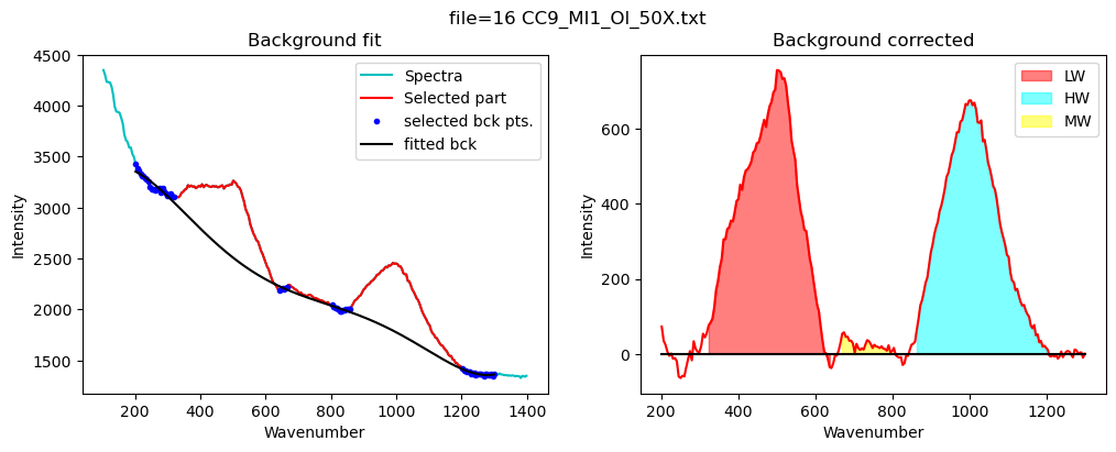
    # Fit silica spectra
    df_sil=pf.fit_area_for_silicate_region(Spectra=Spectra2,
    path=spectra_path, filename=filename_Host, config1=config_silicate,
     plot_figure=True,
    fit_sil='poly')

    data=pf.stitch_dataframes_together(df_sil=df_sil,
        df_water=df_H2O,
Host_file=filename_Host, MI_file=filename_MI)

    df_merged = pd.concat([df_merged, data], axis=0)

df_merged=df_merged.reset_index(drop=True)

100%|██████████| 9/9 [00:06<00:00,  1.40it/s]

# You can inspect the results here
df_merged.head()

	Host filename	MI filename	Water_to_HW_ratio_Trapezoid	Water_to_HW_ratio_Simpson	Water_to_Total_Silicate_ratio_Trapezoid	Water_to_Total_Silicate_ratio_Simpson	Water_Trapezoid_Area	Water_Simpson_Area	Silicate_Trapezoid_Area	Silicate_Simpson_Area	...	HW_Silicate_Trapezoid_Area	HW_Silicate_Simpson_Area	MW_Silicate_Trapezoid_Area	MW_Silicate_Simpson_Area	Water Filename	Water_LHS_Back1	Water_LHS_Back2	Water_RHS_Back1	Water_RHS_Back2	Water_N_Poly
0	03 CC14_MI2_Ol_96mw.txt	02 CC14_MI2_H2O_96mw.txt	1.292630	1.291034	0.556332	0.556073	211330.717146	211165.808780	379864.496263	379745.013178	...	163488.966895	163563.287063	2856.492903	2889.766264	03 CC14_MI2_Ol_96mw.txt	2400	2750	3750	4100	2
1	06 CC13_MI4_Ol.txt	05 CC13_MI4_H2O.txt	1.273932	1.275060	0.540900	0.540831	204905.623402	204953.099115	378823.385237	378959.477396	...	160845.062379	160739.920557	3243.413314	3171.252208	06 CC13_MI4_Ol.txt	2400	2750	3750	4100	2
2	10 CC9_MI3_Ol.txt	09 CC9_MI3_H2O.txt	1.462606	1.464274	0.608228	0.609066	390345.883604	390493.015370	641775.587932	641133.969309	...	266883.839787	266680.342116	8678.840041	8710.813827	10 CC9_MI3_Ol.txt	2400	2750	3750	4100	2
3	16 CC9_MI1_Ol_50X.txt	12 CC9_MI1_H2O_20X.txt	2.295836	2.294857	1.036495	1.036426	271652.008729	271618.716229	262087.178060	262072.519289	...	118323.771655	118359.740987	3076.166398	3017.302181	16 CC9_MI1_Ol_50X.txt	2400	2750	3750	4100	2
4	16 CC9_MI1_Ol_50X.txt	15 CC9_MI1_H2O_50X.txt	1.290089	1.291685	0.585702	0.586346	203547.742283	203697.502551	347528.113007	347401.545257	...	157778.011672	157699.085679	5423.488225	5568.872826	16 CC9_MI1_Ol_50X.txt	2400	2750	3750	4100	2

5 rows × 27 columns

# And save them to Excel here
df_merged.to_excel('H2O_Silicate_areas.xlsx')