This page was generated from docs/Examples/Fitting_Water_Silicate_Melts/Example4a_H2OQuant_Glass/H2O_Fitting.ipynb. Interactive online version: .

Python Notebook Download

Example 4 a- Fitting H2O:Silicate areas in glasses

• This notebook shows how to quantify the relative area of the silicate peak and H2O peak in glasses

• Please see example 4b if you want to quantify H2O/silicate areas in unexposed olivine-hosted melt inclusions

• This folder lets you fit one spectra at a time - this is best if you need to adjust the fits for each spectra. It saves each fit to a CSV, then you go to the end of the notebook and stitch these all together into 1 file.

• There is also an example coming soon for looping through all spectra using the same fit parameters

Install DiadFit if you havent already- uncomment this!

#!pip install --upgrade DiadFit

Import necessary python things

import numpy as np
import pandas as pd
import matplotlib.pyplot as plt
import DiadFit as pf
pf.__version__

'1.0.3'

# Set your ptah here - this assumes the txt files are in the same folder as the notebook, but you can easily add a different directory here. Chat GPT can help you with that!
import os
DayFolder=os.getcwd()
spectra_path=DayFolder
file_ext='.txt'
filetype='headless_txt'

H2O_Files=pf.get_files(path=spectra_path,
file_ext=file_ext, sort=False)
H2O_Files

['ETFS_OL39_MI7_50X_GLASS.txt', 'test_H2O.txt']

### Select file

• Come back to here and change the i value

print('max i value='+str(len(H2O_Files)-1))

max i value=1

i=0
filename_H2O=H2O_Files[i]
print(filename_H2O)

ETFS_OL39_MI7_50X_GLASS.txt

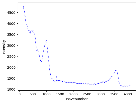
# Plot the spectra from the glass sample collected by Raman
spectra_H2O=pf.get_data(path=spectra_path, filename=filename_H2O,
            Diad_files=None, filetype=filetype)
plt.plot(spectra_H2O[:, 0], spectra_H2O[:,1], ':b')
plt.xlabel('Wavenumber')
plt.ylabel('Intensity')

Text(0, 0.5, 'Intensity')

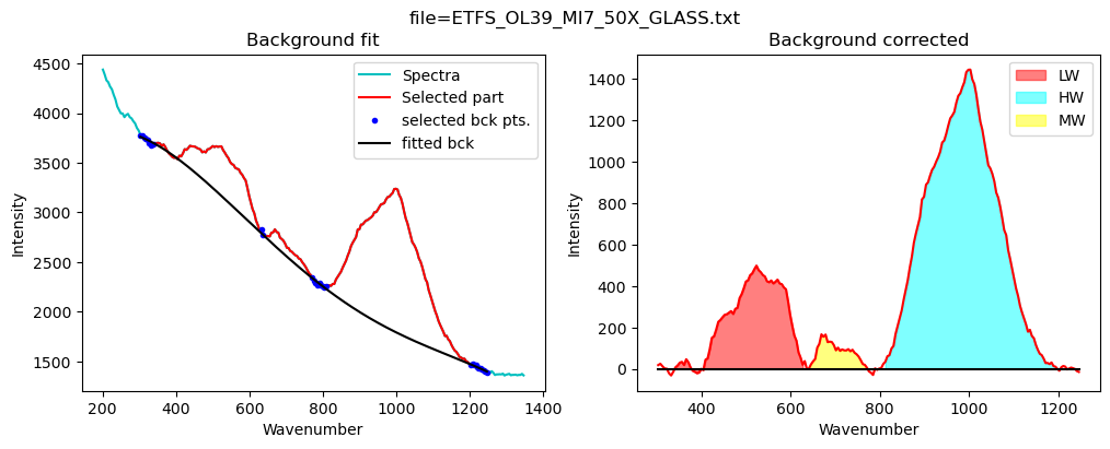
Now lets quantify the area under the silicate region

# We have stored default fit parameters, you can see them here
pf.sil_bck_pos_Schiavi_basalt()

sil_bck_pos_Schiavi_basalt(lower_range_sil=(300, 340), mid_range1_sil=(630, 640), mid_range2_sil=(800, 830), upper_range_sil=(1200, 1250), LW=(400, 600), HW=(800, 1200), N_poly_sil=3, sigma_sil=5)

# You can edit any of them by writing the variable name between these brackets, and entering new numbers that might work better for your system
config_silicate=pf.sil_bck_pos_Schiavi_basalt(mid_range2_sil=(770, 810),
     N_poly_sil=4, LW=(400, 600), HW=(800, 1200))
config_silicate

sil_bck_pos_Schiavi_basalt(lower_range_sil=(300, 340), mid_range1_sil=(630, 640), mid_range2_sil=(770, 810), upper_range_sil=(1200, 1250), LW=(400, 600), HW=(800, 1200), N_poly_sil=4, sigma_sil=5)

# This cell calculates the area under the 3 different silicate regions
df_sil=pf.fit_area_for_silicate_region(Spectra=spectra_H2O,
path=spectra_path, filename=filename_H2O, config1=config_silicate,
exclude_range1_sil=None, exclude_range2_sil=None,  plot_figure=True,
fit_sil='poly')
df_sil

	Silicate_LHS_Back1	Silicate_LHS_Back2	Silicate_RHS_Back1	Silicate_RHS_Back2	Silicate_N_Poly	Silicate_Trapezoid_Area	Silicate_Simpson_Area	LW_Silicate_Trapezoid_Area	LW_Silicate_Simpson_Area	HW_Silicate_Trapezoid_Area	HW_Silicate_Simpson_Area	MW_Silicate_Trapezoid_Area	MW_Silicate_Simpson_Area
0	300	340	1200	1250	4	362558.10011	362437.552216	69943.66401	69904.770625	265265.242676	265018.00209	11333.332933	11224.5619

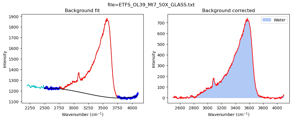
Now quantify the area under the water region

# Again, there is a default set of variables
pf.water_bck_pos()

water_bck_pos(fit_water='poly', N_poly_water=3, lower_bck_water=(2750, 3100), upper_bck_water=(3750, 4100))

# And you can edit any of these values here - we are tweaking the lower background
config_H2O=pf.water_bck_pos(lower_bck_water=(2500, 2750))
print(config_H2O)

df_H2O=pf.fit_area_for_water_region(
path=spectra_path, filename=filename_H2O,
Spectra=spectra_H2O,
config1=config_H2O)
df_H2O

water_bck_pos(fit_water='poly', N_poly_water=3, lower_bck_water=(2500, 2750), upper_bck_water=(3750, 4100))

	Water Filename	Water_LHS_Back1	Water_LHS_Back2	Water_RHS_Back1	Water_RHS_Back2	Water_N_Poly	Water_Trapezoid_Area	Water_Simpson_Area
0	ETFS_OL39_MI7_50X_GLASS.txt	2500	2750	3750	4100	3	274807.39519	274611.003728

# This combines the outputs you got from silicate fitting and H2O fitting.
combo_out=pf.stitch_dataframes_together(df_sil=df_sil, df_water=df_H2O,
MI_file=filename_H2O, save_csv=True, path=DayFolder)
combo_out

	MI filename	Water_to_HW_ratio_Trapezoid	Water_to_HW_ratio_Simpson	Water_to_Total_Silicate_ratio_Trapezoid	Water_to_Total_Silicate_ratio_Simpson	Water_Trapezoid_Area	Water_Simpson_Area	Silicate_Trapezoid_Area	Silicate_Simpson_Area	Silicate_LHS_Back1	...	HW_Silicate_Trapezoid_Area	HW_Silicate_Simpson_Area	MW_Silicate_Trapezoid_Area	MW_Silicate_Simpson_Area	Water Filename	Water_LHS_Back1	Water_LHS_Back2	Water_RHS_Back1	Water_RHS_Back2	Water_N_Poly
0	ETFS_OL39_MI7_50X_GLASS.txt	1.035972	1.036198	0.757968	0.757678	274807.39519	274611.003728	362558.10011	362437.552216	300	...	265265.242676	265018.00209	11333.332933	11224.5619	ETFS_OL39_MI7_50X_GLASS.txt	2500	2750	3750	4100	3

1 rows × 26 columns

You have fitted one file - Now click this to go back to the top and do the next file and so on by changing i

Select file

Once you’ve fitted all your files…

• Now stitch them, this code works by finding Stitching all the files together once you have them

csv_files2=pf.get_files(path=DayFolder, ID_str='combo_fit',
    sort=True, file_ext='csv')
csv_files2

['ETFS_OL39_MI7_50X_GLASS_combo_fit.csv', 'test_H2O_combo_fit.csv']

Stitch data from all these CSVs together

df = pd.concat(
    map(pd.read_csv, csv_files2), ignore_index=True)
df

	Unnamed: 0	MI filename	Water_to_HW_ratio_Trapezoid	Water_to_HW_ratio_Simpson	Water_to_Total_Silicate_ratio_Trapezoid	Water_to_Total_Silicate_ratio_Simpson	Water_Trapezoid_Area	Water_Simpson_Area	Silicate_Trapezoid_Area	Silicate_Simpson_Area	...	MW_Silicate_Trapezoid_Area	MW_Silicate_Simpson_Area	Water Filename	Water_LHS_Back1	Water_LHS_Back2	Water_RHS_Back1	Water_RHS_Back2	Water_N_Poly	HW:LW_Trapezoid	HW:LW_Simpson
0	0	ETFS_OL39_MI7_50X_GLASS.txt	1.035972	1.036198	0.757968	0.757678	274807.39519	274611.003728	362558.10011	362437.552216	...	11333.332933	11224.5619	ETFS_OL39_MI7_50X_GLASS.txt	2500	2750	3750	4100	3	NaN	NaN
1	0	test_H2O.txt	NaN	NaN	NaN	NaN	274807.39519	274611.003728	362558.10011	362437.552216	...	11333.332933	11224.5619	test_H2O.txt	2500	2750	3750	4100	3	3.928982	3.928359

2 rows × 29 columns

Now save to Excel

df.to_excel('H2O_Silicate_areas.xlsx')