This page was generated from
docs/Examples/EOS_calculations/Example5e_FI_Monte_Carlo_Simulations.ipynb.
Interactive online version:
![]() .
.
Propagating uncertainties in fluid inclusion barometry
This notebook shows how to propagate uncertainty when performing fluid inclusion barometry
[12]:
import numpy as np
import pandas as pd
import matplotlib.pyplot as plt
import DiadFit as pf
pf.__version__
[12]:
'1.0.23'
Load in the data
You can call your column headings whatever you want, just swap the text when it references them later
[13]:
# Get from here - https://github.com/PennyWieser/DiadFit/blob/main/docs/Examples/EOS_calculations/Fluid_Inclusion_Densities_Example1.xlsx
df=pd.read_excel('Fluid_Inclusion_Densities_Example1.xlsx', sheet_name='Diff_Temps')
df.head()
[13]:
| Sample | Density_g_cm3 | T_C | XH2O | Host_Fo_content | |
|---|---|---|---|---|---|
| 0 | FI1 | 0.458055 | 1048.898738 | 0.086258 | 0.897797 |
| 1 | FI2 | 0.492947 | 1015.924767 | 0.085212 | 0.831850 |
| 2 | FI4 | 0.484594 | 1041.589916 | 0.085462 | 0.883180 |
| 3 | FI5 | 0.494431 | 1034.935183 | 0.085167 | 0.869870 |
| 4 | FI7 | 0.476416 | 1034.820102 | 0.085708 | 0.869640 |
Propagating uncertainty in temperature
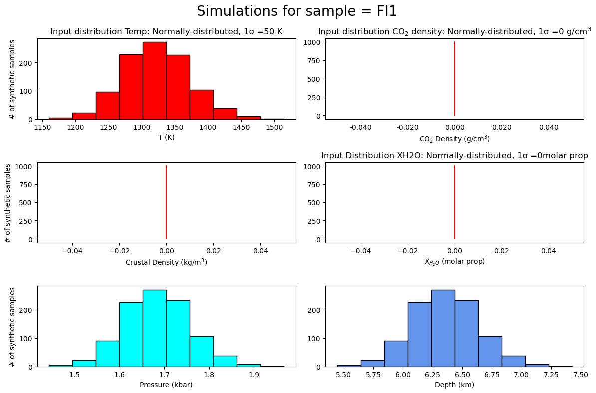
Lets say the uncertainty in temperature is +-50K. So this is an absolute error, and we want temperature distributed normally
We want to use a single step profile initially to convert pressure to depth
We want to make 1000 duplicates per FI with temperature varying by 1 sigma=50K
It outputs MC_Av, which is the average for each fluid inclusion, and MC_All, which contains rows for each of the N duplicates you asked for appended end-on-end
[14]:
MC_Av_Tonly, MC_All_Tonly, fig=pf.propagate_FI_uncertainty(T_K=df['T_C']+273.15,
error_T_K=50, error_type_T_K='Abs', error_dist_T_K='normal',
                        CO2_dens_gcm3=df['Density_g_cm3'],
                        sample_ID=df['Sample'],
                        crust_dens_kgm3=2700, EOS='SW96',
                        N_dup=1000, fig_i=0, plot_figure=True)
MC_Av_Tonly.head()
We are not using multiprocessing based on your selected EOS. You can override this by setting multiprocess=True in the function, but for SP94 and SW96 it might actually be slower
Processing: 100%|██████████| 60/60 [00:00<00:00, 123.50it/s]
[14]:
| Filename | CO2_dens_gcm3 | SingleCalc_D_km | SingleCalc_P_kbar | Mean_MC_P_kbar | Med_MC_P_kbar | std_dev_MC_P_kbar | std_dev_MC_P_kbar_from_percentile | Mean_MC_D_km | Med_MC_D_km | std_dev_MC_D_km | std_dev_MC_D_km_from_percentile | T_K_input | error_T_K | CO2_dens_gcm3_input | error_CO2_dens_gcm3 | crust_dens_kgm3_input | error_crust_dens_kgm3 | model | EOS | |
|---|---|---|---|---|---|---|---|---|---|---|---|---|---|---|---|---|---|---|---|---|
| 0 | FI1 | 0.458055 | 6.357853 | 1.684004 | 1.685797 | 1.686883 | 0.074176 | 0.074742 | 6.364619 | 6.368722 | 0.280047 | 0.282182 | 1322.048738 | 50 | 0.458055 | 0 | 2700 | 0.0 | None | SW96 |
| 1 | FI2 | 0.492947 | 6.918818 | 1.832587 | 1.837667 | 1.838193 | 0.081741 | 0.080940 | 6.937997 | 6.939981 | 0.308606 | 0.305585 | 1289.074767 | 50 | 0.492947 | 0 | 2700 | 0.0 | None | SW96 |
| 2 | FI4 | 0.484594 | 6.891995 | 1.825483 | 1.825939 | 1.830595 | 0.081023 | 0.080949 | 6.893717 | 6.911297 | 0.305898 | 0.305619 | 1314.739916 | 50 | 0.484594 | 0 | 2700 | 0.0 | None | SW96 |
| 3 | FI5 | 0.494431 | 7.071963 | 1.873151 | 1.869800 | 1.870208 | 0.087073 | 0.085887 | 7.059313 | 7.060854 | 0.328737 | 0.324261 | 1308.085183 | 50 | 0.494431 | 0 | 2700 | 0.0 | None | SW96 |
| 4 | FI7 | 0.476416 | 6.670854 | 1.766909 | 1.762232 | 1.763974 | 0.082242 | 0.083643 | 6.653195 | 6.659773 | 0.310498 | 0.315790 | 1307.970102 | 50 | 0.476416 | 0 | 2700 | 0.0 | None | SW96 |
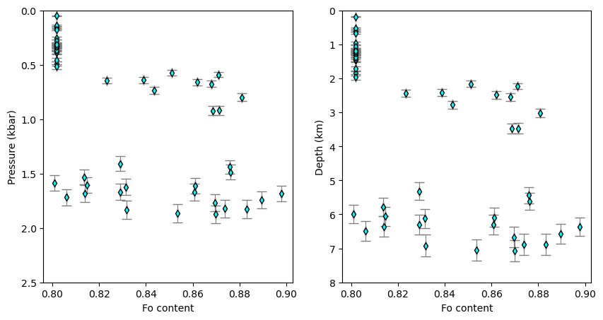
Plot each FI and its 1 sigma error
Lets plot the pressure of the inputted FI (SingleFI_P_kbar), and then the standard deviation of the MC simulation against the Fo content
[15]:
MC_Av_Tonly.head()
[15]:
| Filename | CO2_dens_gcm3 | SingleCalc_D_km | SingleCalc_P_kbar | Mean_MC_P_kbar | Med_MC_P_kbar | std_dev_MC_P_kbar | std_dev_MC_P_kbar_from_percentile | Mean_MC_D_km | Med_MC_D_km | std_dev_MC_D_km | std_dev_MC_D_km_from_percentile | T_K_input | error_T_K | CO2_dens_gcm3_input | error_CO2_dens_gcm3 | crust_dens_kgm3_input | error_crust_dens_kgm3 | model | EOS | |
|---|---|---|---|---|---|---|---|---|---|---|---|---|---|---|---|---|---|---|---|---|
| 0 | FI1 | 0.458055 | 6.357853 | 1.684004 | 1.685797 | 1.686883 | 0.074176 | 0.074742 | 6.364619 | 6.368722 | 0.280047 | 0.282182 | 1322.048738 | 50 | 0.458055 | 0 | 2700 | 0.0 | None | SW96 |
| 1 | FI2 | 0.492947 | 6.918818 | 1.832587 | 1.837667 | 1.838193 | 0.081741 | 0.080940 | 6.937997 | 6.939981 | 0.308606 | 0.305585 | 1289.074767 | 50 | 0.492947 | 0 | 2700 | 0.0 | None | SW96 |
| 2 | FI4 | 0.484594 | 6.891995 | 1.825483 | 1.825939 | 1.830595 | 0.081023 | 0.080949 | 6.893717 | 6.911297 | 0.305898 | 0.305619 | 1314.739916 | 50 | 0.484594 | 0 | 2700 | 0.0 | None | SW96 |
| 3 | FI5 | 0.494431 | 7.071963 | 1.873151 | 1.869800 | 1.870208 | 0.087073 | 0.085887 | 7.059313 | 7.060854 | 0.328737 | 0.324261 | 1308.085183 | 50 | 0.494431 | 0 | 2700 | 0.0 | None | SW96 |
| 4 | FI7 | 0.476416 | 6.670854 | 1.766909 | 1.762232 | 1.763974 | 0.082242 | 0.083643 | 6.653195 | 6.659773 | 0.310498 | 0.315790 | 1307.970102 | 50 | 0.476416 | 0 | 2700 | 0.0 | None | SW96 |
[16]:
fig, (ax1, ax2) = plt.subplots(1, 2, figsize=(10,5))

ax1.errorbar(df['Host_Fo_content'],
             MC_Av_Tonly['SingleCalc_P_kbar'],
             xerr=0, yerr=MC_Av_Tonly['std_dev_MC_P_kbar'],
             fmt='d', ecolor='grey', elinewidth=0.8, mfc='cyan', ms=5, mec='k', capsize=5)

ax1.set_xlabel('Fo content')
ax1.set_ylabel('Pressure (kbar)')

ax2.errorbar(df['Host_Fo_content'],
             MC_Av_Tonly['SingleCalc_D_km'],
             xerr=0, yerr=MC_Av_Tonly['std_dev_MC_D_km'],
             fmt='d', ecolor='grey', elinewidth=0.8, mfc='cyan', ms=5, mec='k', capsize=5)
ax2.set_xlabel('Fo content')
ax2.set_ylabel('Depth (km)')


ax1.set_ylim([0, 2.5])
ax2.set_ylim([0, 8])
ax1.invert_yaxis()
ax2.invert_yaxis()
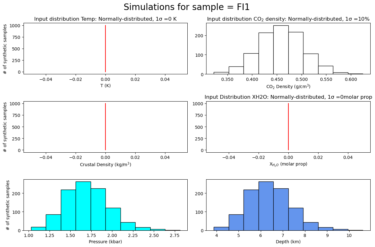
Propagating uncertainty in CO2 Density
Lets say the uncertainty in CO2 density is +-10%, in reality, this will vary greatly between instruments, as well with the absolute density (e.g. more like +-20% for the very weakest diads, more like +-5% for the densest).
[17]:
MC_Av_rhoonly, MC_All_rhoonly, fig=pf.propagate_FI_uncertainty(T_K=df['T_C']+273.15,
error_CO2_dens=10, error_type_CO2_dens='Perc', error_dist_CO2_dens='normal',
                        CO2_dens_gcm3=df['Density_g_cm3'],
                        sample_ID=df['Sample'],
                        crust_dens_kgm3=2700,
                        N_dup=1000, fig_i=0, plot_figure=True)
MC_Av_rhoonly.head()
We are not using multiprocessing based on your selected EOS. You can override this by setting multiprocess=True in the function, but for SP94 and SW96 it might actually be slower
Processing: 100%|██████████| 60/60 [00:00<00:00, 104.56it/s]
[17]:
| Filename | CO2_dens_gcm3 | SingleCalc_D_km | SingleCalc_P_kbar | Mean_MC_P_kbar | Med_MC_P_kbar | std_dev_MC_P_kbar | std_dev_MC_P_kbar_from_percentile | Mean_MC_D_km | Med_MC_D_km | std_dev_MC_D_km | std_dev_MC_D_km_from_percentile | T_K_input | error_T_K | CO2_dens_gcm3_input | error_CO2_dens_gcm3 | crust_dens_kgm3_input | error_crust_dens_kgm3 | model | EOS | |
|---|---|---|---|---|---|---|---|---|---|---|---|---|---|---|---|---|---|---|---|---|
| 0 | FI1 | 0.458055 | 6.357853 | 1.684004 | 1.683790 | 1.653997 | 0.263485 | 0.263253 | 6.357044 | 6.244563 | 0.994773 | 0.993896 | 1322.048738 | 0 | 0.458055 | 10 | 2700 | 0.0 | None | SW96 |
| 1 | FI2 | 0.492947 | 6.918818 | 1.832587 | 1.836499 | 1.828594 | 0.281365 | 0.280905 | 6.933585 | 6.903741 | 1.062275 | 1.060541 | 1289.074767 | 0 | 0.492947 | 10 | 2700 | 0.0 | None | SW96 |
| 2 | FI4 | 0.484594 | 6.891995 | 1.825483 | 1.845013 | 1.832922 | 0.286605 | 0.283461 | 6.965732 | 6.920081 | 1.082059 | 1.070188 | 1314.739916 | 0 | 0.484594 | 10 | 2700 | 0.0 | None | SW96 |
| 3 | FI5 | 0.494431 | 7.071963 | 1.873151 | 1.877689 | 1.867808 | 0.298490 | 0.295090 | 7.089098 | 7.051791 | 1.126929 | 1.114094 | 1308.085183 | 0 | 0.494431 | 10 | 2700 | 0.0 | None | SW96 |
| 4 | FI7 | 0.476416 | 6.670854 | 1.766909 | 1.770855 | 1.752965 | 0.281408 | 0.285410 | 6.685753 | 6.618210 | 1.062440 | 1.077547 | 1307.970102 | 0 | 0.476416 | 10 | 2700 | 0.0 | None | SW96 |
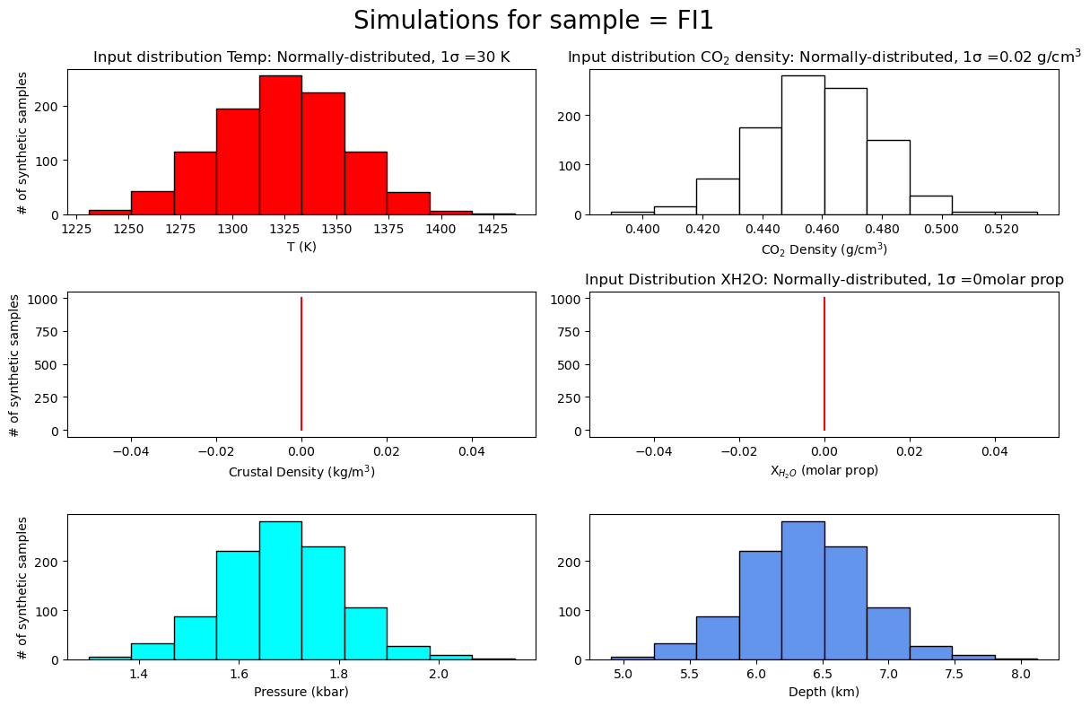
Simulation varying both temperature and CO\(_2\) density
Lets say you think you have +-30K uncertainty in temp, and +-0.02 g/cm3 in density
[18]:
MC_Av_rho_T, MC_All_rho_T, fig=pf.propagate_FI_uncertainty(
T_K=df['T_C']+273.15,
error_CO2_dens=0.02, error_type_CO2_dens='Abs', error_dist_CO2_dens='normal',
error_T_K=30, error_type_T_K='Abs', error_dist_T_K='normal',
CO2_dens_gcm3=df['Density_g_cm3'],
sample_ID=df['Sample'],
crust_dens_kgm3=2700,
N_dup=1000, fig_i=0, plot_figure=True)
MC_Av_rho_T.head()
We are not using multiprocessing based on your selected EOS. You can override this by setting multiprocess=True in the function, but for SP94 and SW96 it might actually be slower
Processing: 100%|██████████| 60/60 [00:00<00:00, 124.29it/s]
[18]:
| Filename | CO2_dens_gcm3 | SingleCalc_D_km | SingleCalc_P_kbar | Mean_MC_P_kbar | Med_MC_P_kbar | std_dev_MC_P_kbar | std_dev_MC_P_kbar_from_percentile | Mean_MC_D_km | Med_MC_D_km | std_dev_MC_D_km | std_dev_MC_D_km_from_percentile | T_K_input | error_T_K | CO2_dens_gcm3_input | error_CO2_dens_gcm3 | crust_dens_kgm3_input | error_crust_dens_kgm3 | model | EOS | |
|---|---|---|---|---|---|---|---|---|---|---|---|---|---|---|---|---|---|---|---|---|
| 0 | FI1 | 0.458055 | 6.357853 | 1.684004 | 1.685454 | 1.682366 | 0.120040 | 0.119029 | 6.363327 | 6.351667 | 0.453203 | 0.449387 | 1322.048738 | 30 | 0.458055 | 0.02 | 2700 | 0.0 | None | SW96 |
| 1 | FI2 | 0.492947 | 6.918818 | 1.832587 | 1.838318 | 1.842039 | 0.122191 | 0.120655 | 6.940455 | 6.954502 | 0.461324 | 0.455527 | 1289.074767 | 30 | 0.492947 | 0.02 | 2700 | 0.0 | None | SW96 |
| 2 | FI4 | 0.484594 | 6.891995 | 1.825483 | 1.826517 | 1.821858 | 0.123161 | 0.125105 | 6.895898 | 6.878309 | 0.464988 | 0.472328 | 1314.739916 | 30 | 0.484594 | 0.02 | 2700 | 0.0 | None | SW96 |
| 3 | FI5 | 0.494431 | 7.071963 | 1.873151 | 1.877447 | 1.870149 | 0.130848 | 0.123279 | 7.088184 | 7.060629 | 0.494009 | 0.465430 | 1308.085183 | 30 | 0.494431 | 0.02 | 2700 | 0.0 | None | SW96 |
| 4 | FI7 | 0.476416 | 6.670854 | 1.766909 | 1.765907 | 1.765243 | 0.122329 | 0.118946 | 6.667069 | 6.664565 | 0.461847 | 0.449072 | 1307.970102 | 30 | 0.476416 | 0.02 | 2700 | 0.0 | None | SW96 |
Uncertainty in Temp, CO2 and Crustal density
Here we also add a 5% uncertainty in crustal density.
[19]:
MC_Av_rho_T_CD, MC_All_rho_T_CD, fig=pf.propagate_FI_uncertainty(T_K=df['T_C']+273.15,
error_CO2_dens=0.02, error_type_CO2_dens='Abs', error_dist_CO2_dens='normal',
error_T_K=30, error_type_T_K='Abs', error_dist_T_K='normal',
crust_dens_kgm3=2700,
error_crust_dens=5, error_type_crust_dens='Perc', error_dist_crust_dens='normal',
CO2_dens_gcm3=df['Density_g_cm3'],
sample_ID=df['Sample'],
N_dup=1000, fig_i=0, plot_figure=True )


fig.savefig('MonteCarlo_Sample1_png', dpi=300)
We are not using multiprocessing based on your selected EOS. You can override this by setting multiprocess=True in the function, but for SP94 and SW96 it might actually be slower
Processing: 100%|██████████| 60/60 [00:00<00:00, 85.71it/s]

[20]:
MC_Av_rho_T_CD.head()
[20]:
| Filename | CO2_dens_gcm3 | SingleCalc_D_km | SingleCalc_P_kbar | Mean_MC_P_kbar | Med_MC_P_kbar | std_dev_MC_P_kbar | std_dev_MC_P_kbar_from_percentile | Mean_MC_D_km | Med_MC_D_km | std_dev_MC_D_km | std_dev_MC_D_km_from_percentile | T_K_input | error_T_K | CO2_dens_gcm3_input | error_CO2_dens_gcm3 | crust_dens_kgm3_input | error_crust_dens_kgm3 | model | EOS | |
|---|---|---|---|---|---|---|---|---|---|---|---|---|---|---|---|---|---|---|---|---|
| 0 | FI1 | 0.458055 | 6.357853 | 1.684004 | 1.685074 | 1.685617 | 0.124671 | 0.123585 | 6.374555 | 6.366292 | 0.570062 | 0.578528 | 1322.048738 | 30 | 0.458055 | 0.02 | 2700 | 5.0 | None | SW96 |
| 1 | FI2 | 0.492947 | 6.918818 | 1.832587 | 1.832410 | 1.822413 | 0.135376 | 0.137487 | 6.934632 | 6.919253 | 0.633050 | 0.676458 | 1289.074767 | 30 | 0.492947 | 0.02 | 2700 | 5.0 | None | SW96 |
| 2 | FI4 | 0.484594 | 6.891995 | 1.825483 | 1.825434 | 1.821722 | 0.124641 | 0.119349 | 6.902983 | 6.881754 | 0.594297 | 0.569676 | 1314.739916 | 30 | 0.484594 | 0.02 | 2700 | 5.0 | None | SW96 |
| 3 | FI5 | 0.494431 | 7.071963 | 1.873151 | 1.874703 | 1.871307 | 0.131854 | 0.133520 | 7.075627 | 7.061422 | 0.609445 | 0.607685 | 1308.085183 | 30 | 0.494431 | 0.02 | 2700 | 5.0 | None | SW96 |
| 4 | FI7 | 0.476416 | 6.670854 | 1.766909 | 1.772892 | 1.764315 | 0.123605 | 0.124702 | 6.689497 | 6.666561 | 0.566341 | 0.564543 | 1307.970102 | 30 | 0.476416 | 0.02 | 2700 | 5.0 | None | SW96 |
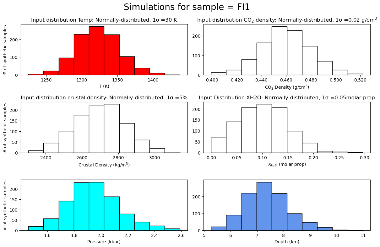
Uncertainty in Temp, CO2 density, crustal density and XH2O
If XH2O is not None, the function will use the EOS of Duan and Zhang (2006) to propagate this additional source of uncertainty. Note, these calculations are an order of magnitude slower, so it may take several minutes to run. We are using multiprocessing to speed it up.
Here we consider XH2O=0.1, with a uniformly distributed error of +-0.05
[21]:
MC_Av_rho_T_CDH, MC_All_rho_T_CDH, fig=pf.propagate_FI_uncertainty(T_K=df['T_C']+273.15,
error_CO2_dens=0.02, error_type_CO2_dens='Abs', error_dist_CO2_dens='normal',
error_T_K=30, error_type_T_K='Abs', error_dist_T_K='normal',
crust_dens_kgm3=2700,
error_crust_dens=5, error_type_crust_dens='Perc', error_dist_crust_dens='normal',
CO2_dens_gcm3=df['Density_g_cm3'],
XH2O=0.1, error_XH2O=0.05, error_type_XH2O='Abs', error_dist_XH2O='normal',
sample_ID=df['Sample'],
N_dup=1000, fig_i=0, plot_figure=True )
MC_Av_rho_T_CDH.head()
You have entered a value for XH2O, so we are now using the EOS of Duan and Zhang 200 regardless of what model you selected. If you dont want this, specify XH2O=None
Please note, the DZ2006 EOS is about 5-40X slower to run than the SP94 and SW94 EOS
We are using multiprocessing based on your selected EOS. You can override this by setting multiprocess=False in the function, but it might slow it down a lot
Number of processors:  8
[21]:
| Filename | i | CO2_density_input | SingleCalc_D_km | SingleCalc_P_kbar | Mean_MC_P_kbar | Med_MC_P_kbar | std_dev_MC_P_kbar | std_dev_MC_P_kbar_from_percentile | Mean_MC_D_km | ... | T_K_input | error_T_K | CO2_dens_gcm3_input | error_CO2_dens_gcm3 | crust_dens_kgm3_input | error_crust_dens_kgm3 | model | EOS | XH2O_input | error_XH2O | |
|---|---|---|---|---|---|---|---|---|---|---|---|---|---|---|---|---|---|---|---|---|---|
| 0 | FI1 | 0.0 | 0.458055 | 7.291610 | 1.931329 | 1.946028 | 1.935574 | 0.192155 | 0.182582 | 7.374642 | ... | 1322.048738 | 30.0 | 0.458055 | 0.02 | 2700.0 | 5.0 | None | DZ06 | 0.1 | 0.05 |
| 1 | FI2 | 1.0 | 0.492947 | 7.905409 | 2.093906 | 2.121787 | 2.098956 | 0.212000 | 0.205083 | 8.040700 | ... | 1289.074767 | 30.0 | 0.492947 | 0.02 | 2700.0 | 5.0 | None | DZ06 | 0.1 | 0.05 |
| 2 | FI4 | 2.0 | 0.484594 | 7.869712 | 2.084451 | 2.112670 | 2.089794 | 0.210073 | 0.202420 | 8.006136 | ... | 1314.739916 | 30.0 | 0.484594 | 0.02 | 2700.0 | 5.0 | None | DZ06 | 0.1 | 0.05 |
| 3 | FI5 | 3.0 | 0.494431 | 8.089363 | 2.142630 | 2.170117 | 2.148561 | 0.216681 | 0.209704 | 8.223869 | ... | 1308.085183 | 30.0 | 0.494431 | 0.02 | 2700.0 | 5.0 | None | DZ06 | 0.1 | 0.05 |
| 4 | FI7 | 4.0 | 0.476416 | 7.601455 | 2.013397 | 2.043449 | 2.019502 | 0.202435 | 0.195015 | 7.743774 | ... | 1307.970102 | 30.0 | 0.476416 | 0.02 | 2700.0 | 5.0 | None | DZ06 | 0.1 | 0.05 |
5 rows × 23 columns
[22]:
fig.savefig('MC for paper.png', dpi=300)
[ ]: