This page was generated from
docs/Examples/EOS_calculations/Example5d_Fluid_Inclusion_Density_to_Depth.ipynb.
Interactive online version:
![]() .
.
Converting CO2 densities to pressures to depths
This notebook shows how to use the equation of state of pure CO2 of Span and Wanger (1996) implemented through coolprop to calculate pressures of fluid inclusions
We also show how to use Monte-Carlo simulations to propagate errors when determing fluid inclusion pressures
We also show how to calculate densities to depths using a variety of crustal density models
See the notebook ‘Dayton_et_al_2023_LaPalmaExample.ipynb’ to see how to propagate uncertainty in these different parameters
Install DiadFit if you havent already! You might also have to install CoolProp if you want to use Span and Wagner EOS - the error message will give you instructions, else reach out
[1]:
#!pip install --upgrade DiadFit
First, import all the python things you need
[2]:
import numpy as np
import pandas as pd
import matplotlib.pyplot as plt
import DiadFit as pf
pf.__version__
[2]:
'1.0.11'
Lets just look at a single FI first
[10]:
P_kbar=pf.calculate_P_for_rho_T(T_K=1150+273.15,
CO2_dens_gcm3=0.9)
P_kbar.head()
[10]:
| P_kbar | P_MPa | T_K | CO2_dens_gcm3 | |
|---|---|---|---|---|
| 0 | 6.401596 | 640.159635 | 1423.15 | 0.9 |
[11]:
D_Constant_rho=pf.convert_co2_dens_press_depth(T_K=1150+273.15,
CO2_dens_gcm3=0.9, crust_dens_kgm3=2700, g=9.81, output='df')
D_Constant_rho.head()
[11]:
| Pressure (kbar) | Pressure (MPa) | Depth (km) | MC_crust_dens_kgm3 | model | MC_T_K | MC_CO2_dens_gcm3 | |
|---|---|---|---|---|---|---|---|
| 0 | 6.401596 | 640.159635 | 24.168824 | 2700 | None | 1423.15 | 0.9 |
Load your FI densities
In this example, we just load a simple spreadsheet with densities and a sample name. E.g. this could be from microthermometry, or from Raman
[3]:
# Get from here: https://github.com/PennyWieser/DiadFit/blob/main/docs/Examples/EOS_calculations/Fluid_Inclusion_Densities_Example1.xlsx
data=pd.read_excel('Fluid_Inclusion_Densities_Example1.xlsx')
data.head()
[3]:
| Sample | Density_g_cm3 | |
|---|---|---|
| 0 | FI1 | 0.389845 |
| 1 | FI2 | 0.923179 |
| 2 | FI4 | 0.393791 |
| 3 | FI5 | 0.769280 |
| 4 | FI7 | 0.741868 |
Simple conversion to pressure
Most simply, you can convert each density to pressure using the equation of state of Span and Wagner, implemented in CoolProp.
You also need an estimate of the entrapment temperature. Here we use a fixed value, but you could also allocate a temperature based on the forsterite content of your olivine, or any other thermometer suitable for your system
Temperature must be in Kelvin!
[4]:
P_kbar=pf.calculate_P_for_rho_T(T_K=1150+273.15,
CO2_dens_gcm3=data['Density_g_cm3'])
P_kbar.head()
[4]:
| P_kbar | P_MPa | T_K | CO2_dens_gcm3 | |
|---|---|---|---|---|
| 0 | 1.445991 | 144.599143 | 1423.15 | 0.389845 |
| 1 | 6.780995 | 678.099451 | 1423.15 | 0.923179 |
| 2 | 1.466838 | 146.683822 | 1423.15 | 0.393791 |
| 3 | 4.570341 | 457.034146 | 1423.15 | 0.769280 |
| 4 | 4.246948 | 424.694773 | 1423.15 | 0.741868 |
Convert to Depth in a single step from density
We can also specify a variety of options in this function to directly get depth, instead of pressure
Using a constant crustal density of 2700 kg/m\(^{3}\)
[5]:
D_Constant_rho=pf.convert_co2_dens_press_depth(T_K=1150+273.15,
CO2_dens_gcm3=data['Density_g_cm3'], crust_dens_kgm3=2700, g=9.81, output='df')
D_Constant_rho.head()
[5]:
| Pressure (kbar) | Pressure (MPa) | Depth (km) | MC_crust_dens_kgm3 | model | MC_T_K | MC_CO2_dens_gcm3 | |
|---|---|---|---|---|---|---|---|
| 0 | 1.445991 | 144.599143 | 5.459250 | 2700 | None | 1423.15 | 0.389845 |
| 1 | 6.780995 | 678.099451 | 25.601218 | 2700 | None | 1423.15 | 0.923179 |
| 2 | 1.466838 | 146.683822 | 5.537955 | 2700 | None | 1423.15 | 0.393791 |
| 3 | 4.570341 | 457.034146 | 17.255036 | 2700 | None | 1423.15 | 0.769280 |
| 4 | 4.246948 | 424.694773 | 16.034084 | 2700 | None | 1423.15 | 0.741868 |
Using a two-step crustal density
For this, specify a density above and below a boundary, e.g. volcanic pile vs. oceanic crust in an OIB, or crust vs mantle

[6]:
D_2_step=pf.convert_co2_dens_press_depth(T_K=1150+273.15,
CO2_dens_gcm3=data['Density_g_cm3'], model='two-step', rho1=2600, rho2=3000, d1=5, g=9.81, output='df')
D_2_step.head()
[6]:
| Pressure (kbar) | Pressure (MPa) | Depth (km) | MC_crust_dens_kgm3 | model | MC_T_K | MC_CO2_dens_gcm3 | |
|---|---|---|---|---|---|---|---|
| 0 | 1.445991 | 144.599143 | 5.579991 | None | two-step | 1423.15 | 0.389845 |
| 1 | 6.780995 | 678.099451 | 23.707763 | None | two-step | 1423.15 | 0.923179 |
| 2 | 1.466838 | 146.683822 | 5.650826 | None | two-step | 1423.15 | 0.393791 |
| 3 | 4.570341 | 457.034146 | 16.196199 | None | two-step | 1423.15 | 0.769280 |
| 4 | 4.246948 | 424.694773 | 15.097342 | None | two-step | 1423.15 | 0.741868 |
Using a 3-step crustal density
Here, we assume a volcanic layer, oceanic crust, and mantle.

[7]:
D_3_step=pf.convert_co2_dens_press_depth(T_K=1150+273.15,
CO2_dens_gcm3=data['Density_g_cm3'], model='three-step', rho1=2600, rho2=3000, rho3=3300,
d1=5, d2=14, g=9.81, output='df')
D_3_step.head()
[7]:
| Pressure (kbar) | Pressure (MPa) | Depth (km) | MC_crust_dens_kgm3 | model | MC_T_K | MC_CO2_dens_gcm3 | |
|---|---|---|---|---|---|---|---|
| 0 | 1.445991 | 144.599143 | 5.579991 | None | three-step | 1423.15 | 0.389845 |
| 1 | 6.780995 | 678.099451 | 22.825239 | None | three-step | 1423.15 | 0.923179 |
| 2 | 1.466838 | 146.683822 | 5.650826 | None | three-step | 1423.15 | 0.393791 |
| 3 | 4.570341 | 457.034146 | 15.996545 | None | three-step | 1423.15 | 0.769280 |
| 4 | 4.246948 | 424.694773 | 14.997584 | None | three-step | 1423.15 | 0.741868 |
Using published density profiles - get more detail in the docs
We also include the following crustal density profiles
ryan_lerner: update of Ryan 1987 by Lerner et al. 2021
mavko_debari - Mavko and Thompson (1983) and DeBari and Greene (2011) from Putirka (2017)
hill_zucca - Hill and Zucca (1987) from Putirka (2017)
prezzi - tweaked for andes, Prezzi et al. (2009) from Putirka (2017)
rasmussen - Rasmussen et al. (2022) for arcs
[8]:
D_Ras=pf.convert_co2_dens_press_depth(T_K=1150+273.15,
CO2_dens_gcm3=data['Density_g_cm3'], model='rasmussen', output='df')
D_Ras.head()
[8]:
| Pressure (kbar) | Pressure (MPa) | Depth (km) | MC_crust_dens_kgm3 | model | MC_T_K | MC_CO2_dens_gcm3 | |
|---|---|---|---|---|---|---|---|
| 0 | 1.445991 | 144.599143 | 5.840007 | None | rasmussen | 1423.15 | 0.389845 |
| 1 | 6.780995 | 678.099451 | NaN | None | rasmussen | 1423.15 | 0.923179 |
| 2 | 1.466838 | 146.683822 | 5.920451 | None | rasmussen | 1423.15 | 0.393791 |
| 3 | 4.570341 | 457.034146 | 17.520428 | None | rasmussen | 1423.15 | 0.769280 |
| 4 | 4.246948 | 424.694773 | 16.329165 | None | rasmussen | 1423.15 | 0.741868 |
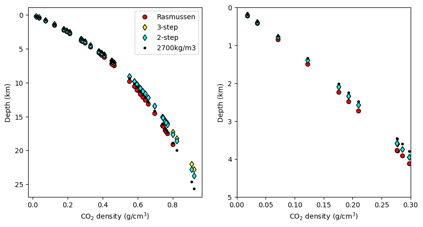
Plot these up to see the differences
[9]:
fig, (ax1, ax2) = plt.subplots(1, 2, figsize=(10,5))
ax1.plot(D_Ras['MC_CO2_dens_gcm3'], D_Ras['Depth (km)'],
         'ok', mfc='red', label='Rasmussen')
ax1.plot(D_3_step['MC_CO2_dens_gcm3'], D_3_step['Depth (km)'],
         'dk', mfc='yellow', label='3-step')
ax1.plot(D_2_step['MC_CO2_dens_gcm3'], D_2_step['Depth (km)'],
         'dk', mfc='cyan', label='2-step')
ax1.plot(D_Constant_rho['MC_CO2_dens_gcm3'], D_Constant_rho['Depth (km)'],
         '.k', mfc='black', label='2700kg/m3')


ax2.plot(D_Ras['MC_CO2_dens_gcm3'], D_Ras['Depth (km)'],
         'ok', mfc='red', label='Rasmussen')
ax2.plot(D_3_step['MC_CO2_dens_gcm3'], D_3_step['Depth (km)'],
         'dk', mfc='yellow', label='3-step')
ax2.plot(D_2_step['MC_CO2_dens_gcm3'], D_2_step['Depth (km)'],
         'dk', mfc='cyan', label='2-step')
ax2.plot(D_Constant_rho['MC_CO2_dens_gcm3'], D_Constant_rho['Depth (km)'],
         '.k', mfc='black', label='2700kg/m3')
ax2.set_xlim([0, 0.3])
ax2.set_ylim([0, 5])

ax1.legend()
ax1.invert_yaxis()
ax2.invert_yaxis()


ax1.set_xlabel('CO$_2$ density (g/cm$^{3}$)')
ax1.set_ylabel('Depth (km)')
ax2.set_xlabel('CO$_2$ density (g/cm$^{3}$)')
ax2.set_ylabel('Depth (km)')
[9]:
Text(0, 0.5, 'Depth (km)')