This page was generated from docs/Examples/EOS_calculations/Example5c_LaPalma_FluidInclusions.ipynb. Interactive online version: .

Python Notebook Download

Example from La Palma

• This notebook shows how to convert the Raman-based FI densities from Dayton et al. (2023) into pressures and depths in the crust

• This assumes +-50K error in entrapment temperature, and an error in CO2 density of 0.002925 g/cm3

• Depth is calculated using a 2-step density profile, with 2.8 g/cm3 above the Moho, and 3.1 g/cm3 below

• You can download the excel spreadsheet here.

• https://github.com/PennyWieser/DiadFit/blob/main/docs/Examples/EOS_calculations/Dayton_et_al_2023_LaPalma_Example.xlsx

Install DiadFit if you havent already! You might also have to install CoolProp if you want to use Span and Wagner EOS - the error message will give you instructions, else reach out

#!pip install --upgrade DiadFit

import pandas as pd
import numpy as np
import matplotlib.pyplot as plt
import DiadFit as pf
pf.__version__

'0.0.91'

Lets load in the data

# Get from here: https://github.com/PennyWieser/DiadFit/blob/main/docs/Examples/EOS_calculations/Dayton_et_al_2023_LaPalma_Example.xlsx
data=pd.read_excel('Dayton_et_al_2023_LaPalma_Example.xlsx',
                   sheet_name='Sheet1')
data.head()

	SAMPLE	FileName	Density (g/cm^3)	Comment (EPMA Data Point)	Na2O	MgO	SiO2	Al2O3	P2O5	K2O	CaO	TiO2	FeO	MnO	Cr2O3	NiO	Total	Fo
0	0	03 LM0 G1 FI1	0.875343	LM0_G1_RIM	0.009036	42.12351	39.90642	0.018331	0.000023	0.005965	0.213926	0.034901	17.91823	0.292019	0.078602	0.190220	100.7912	0.807341
1	0	06 LM0 G2 FI1	0.780430	LM0_G2_CENTER	0.009698	44.42279	39.70696	0.008494	0.000023	0.000412	0.322745	0.022287	15.26419	0.225410	0.018465	0.194827	100.1963	0.838388
2	0	17 LM0 G3 FI3	0.936785	LM0_G3_CENTER	0.011004	45.31343	40.64921	0.016474	0.000023	0.003951	0.241455	0.018161	14.36721	0.216594	0.065003	0.260763	101.1633	0.848989
3	0	11 LM0 G3 FI1 (CRR)	0.928828	LM0_G3_CENTER	0.011004	45.31343	40.64921	0.016474	0.000023	0.003951	0.241455	0.018161	14.36721	0.216594	0.065003	0.260763	101.1633	0.848989
4	0	19 LM0 G3 FI4	0.928514	LM0_G3_CENTER	0.011004	45.31343	40.64921	0.016474	0.000023	0.003951	0.241455	0.018161	14.36721	0.216594	0.065003	0.260763	101.1633	0.848989

plt.hist(data['Density (g/cm^3)'], ec='k')
plt.xlabel('CO$_2$ density (g/cm^3)')
plt.ylabel('# of meas')

Text(0, 0.5, '# of meas')

Now lets propagate uncertainty in each fluid inclusion

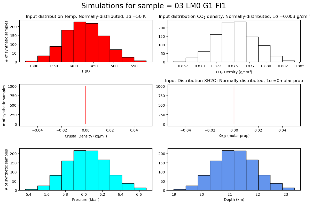
• Here we use a temperature of 1150 K, with a +-50 K (i.e. an absolute uncertainty) distributed normally

• We say the error in CO2 density (from repeated Raman measurements) is 0.002925 g/cm3 (i.e. an absolute uncertainty) distributed normally

• We want to use 2 step crustal density model, with 2800 kg/m3 above 14km depth, and 3100kg/m3 below. Right now, we are not propagating uncertainty in this.

• The figure shows us the simulation file the 1st file (file_i=0). For the Nth file, enter file_i=N-1 as python counting starts at 0

MC_Av, MC_All, fig=pf.propagate_FI_uncertainty(
T_K=1150+273.15,
error_T_K=50,
error_type_T_K='Abs',
error_dist_T_K='normal',
CO2_dens_gcm3=data['Density (g/cm^3)'],
error_CO2_dens=0.002925, error_type_CO2_dens='Abs', error_dist_CO2_dens='normal',
sample_ID=data['FileName'],
model='two-step', d1=14, rho1=2800, rho2=3100,
N_dup=1000, fig_i=0, plot_figure=True)
MC_Av.head()

We are not using multiprocessing based on your selected EOS. You can override this by setting multiprocess=True in the function, but for SP94 and SW96 it might actually be slower

Processing: 100%|██████████| 115/115 [00:01<00:00, 76.97it/s]

	Filename	CO2_dens_gcm3	SingleCalc_D_km	SingleCalc_P_kbar	Mean_MC_P_kbar	Med_MC_P_kbar	std_dev_MC_P_kbar	std_dev_MC_P_kbar_from_percentile	Mean_MC_D_km	Med_MC_D_km	std_dev_MC_D_km	std_dev_MC_D_km_from_percentile	T_K_input	error_T_K	CO2_dens_gcm3_input	error_CO2_dens_gcm3	crust_dens_kgm3_input	error_crust_dens_kgm3	model	EOS
0	03 LM0 G1 FI1	0.875343	21.140399	6.016987	6.031485	6.026854	0.222039	0.219125	21.188075	21.172847	0.730127	0.720544	1423.15	50	0.875343	0.002925	None	0.0	two-step	SW96
1	06 LM0 G2 FI1	0.780430	16.834446	4.707503	4.714673	4.712628	0.187193	0.188277	16.858021	16.851298	0.615543	0.619108	1423.15	50	0.780430	0.002925	None	0.0	two-step	SW96
2	17 LM0 G3 FI3	0.936785	24.412263	7.011993	7.020079	7.023037	0.259320	0.266165	24.438851	24.448577	0.852716	0.875226	1423.15	50	0.936785	0.002925	None	0.0	two-step	SW96
3	11 LM0 G3 FI1 (CRR)	0.928828	23.965558	6.876146	6.870309	6.867972	0.247936	0.246916	23.946364	23.938680	0.815284	0.811931	1423.15	50	0.928828	0.002925	None	0.0	two-step	SW96
4	19 LM0 G3 FI4	0.928514	23.948123	6.870844	6.869369	6.874090	0.253193	0.259509	23.943273	23.958798	0.832571	0.853339	1423.15	50	0.928514	0.002925	None	0.0	two-step	SW96

# This returns 2 dataframes, one showing the mean and standard deviation of the simulation for each fluid inclusion
MC_Av.head()

	Filename	CO2_dens_gcm3	SingleCalc_D_km	SingleCalc_P_kbar	Mean_MC_P_kbar	Med_MC_P_kbar	std_dev_MC_P_kbar	std_dev_MC_P_kbar_from_percentile	Mean_MC_D_km	Med_MC_D_km	std_dev_MC_D_km	std_dev_MC_D_km_from_percentile	T_K_input	error_T_K	CO2_dens_gcm3_input	error_CO2_dens_gcm3	crust_dens_kgm3_input	error_crust_dens_kgm3	model	EOS
0	03 LM0 G1 FI1	0.875343	21.140399	6.016987	6.031485	6.026854	0.222039	0.219125	21.188075	21.172847	0.730127	0.720544	1423.15	50	0.875343	0.002925	None	0.0	two-step	SW96
1	06 LM0 G2 FI1	0.780430	16.834446	4.707503	4.714673	4.712628	0.187193	0.188277	16.858021	16.851298	0.615543	0.619108	1423.15	50	0.780430	0.002925	None	0.0	two-step	SW96
2	17 LM0 G3 FI3	0.936785	24.412263	7.011993	7.020079	7.023037	0.259320	0.266165	24.438851	24.448577	0.852716	0.875226	1423.15	50	0.936785	0.002925	None	0.0	two-step	SW96
3	11 LM0 G3 FI1 (CRR)	0.928828	23.965558	6.876146	6.870309	6.867972	0.247936	0.246916	23.946364	23.938680	0.815284	0.811931	1423.15	50	0.928828	0.002925	None	0.0	two-step	SW96
4	19 LM0 G3 FI4	0.928514	23.948123	6.870844	6.869369	6.874090	0.253193	0.259509	23.943273	23.958798	0.832571	0.853339	1423.15	50	0.928514	0.002925	None	0.0	two-step	SW96

# The second output shows every single simulation for each FI. So the first N rows are for the first FI, then next N rows for the next, etc.
MC_All.head()

	Filename	Pressure (kbar)	Pressure (MPa)	Depth (km)	MC_crust_dens_kgm3	model	MC_T_K	MC_CO2_dens_gcm3
0	03 LM0 G1 FI1	6.121520	612.151979	21.484133	None	two-step	1456.265617	0.872784
1	03 LM0 G1 FI1	5.747624	574.762434	20.254659	None	two-step	1364.131195	0.874644
2	03 LM0 G1 FI1	6.452705	645.270453	22.573163	None	two-step	1508.484791	0.879484
3	03 LM0 G1 FI1	6.292424	629.242358	22.046114	None	two-step	1482.444938	0.876493
4	03 LM0 G1 FI1	6.435249	643.524923	22.515765	None	two-step	1517.705758	0.875919

Lets segment for the eruption sample

• These are ‘Logicals’ e.g. a list of True and False statements, these allow us to splice up the dataframe for each sample

sam0=data['SAMPLE']==0 # this gives a list of true and false for sample = 0
sam1=data['SAMPLE']==2
sam4=data['SAMPLE']==4
sam6=data['SAMPLE']==6

## For example, lets get the data for sample 6
data.loc[sam6].head()

	SAMPLE	FileName	Density (g/cm^3)	Comment (EPMA Data Point)	Na2O	MgO	SiO2	Al2O3	P2O5	K2O	CaO	TiO2	FeO	MnO	Cr2O3	NiO	Total	Fo
90	6	01 LM6 G1 FI1	0.833430	LM6_G1_CORE2	0.000013	41.97921	39.79742	0.016172	0.000023	0.000012	0.244621	0.039359	18.16324	0.289626	0.025383	0.200139	100.7552	0.804681
91	6	07 LM6 G1 FI4	0.831903	LM6_G1_CORE3	0.007265	41.50474	40.45826	0.021972	0.000023	0.001032	0.254588	0.019733	17.99747	0.307189	0.015767	0.176755	100.7648	0.804335
92	6	03 LM6 G1 FI2	0.879573	LM6_G1_NEARMI	0.019585	41.74017	39.96414	0.049670	0.000023	0.004542	0.251532	0.040087	18.45561	0.240858	0.020140	0.172209	100.9586	0.801251
93	6	05 LM6 G1 FI3	0.796166	LM6_G1_NEARMI	0.019585	41.74017	39.96414	0.049670	0.000023	0.004542	0.251532	0.040087	18.45561	0.240858	0.020140	0.172209	100.9586	0.801251
94	6	72 LM6 G10 FI1	0.848642	LM6_G10_CENTER	0.045207	42.88505	40.72833	0.171445	0.019677	0.014681	0.371840	0.060140	17.00363	0.246182	0.000881	0.212640	101.7597	0.818041

Lets plot each FI depth and its error bar, colored by sample (as in Dayton et al. 2023)

fig, (ax1) = plt.subplots(1, 1, figsize=(6,5))


ms=7
# This plots a symbol with its error bar for sample 0
ax1.errorbar(data['Fo'].loc[sam0],
             MC_Av['SingleCalc_D_km'].loc[sam0],
             xerr=0, yerr=MC_Av['std_dev_MC_D_km_from_percentile'].loc[sam0],
             fmt='o', ecolor='k', elinewidth=0.8, mfc='red', ms=ms, mec='k', capsize=5)

# This plots a symbol with its error bar for sample 1
ax1.errorbar(data['Fo'].loc[sam1],
             MC_Av['SingleCalc_D_km'].loc[sam1],
             xerr=0, yerr=MC_Av['std_dev_MC_D_km_from_percentile'].loc[sam1],
             fmt='^', ecolor='k', elinewidth=0.8, mfc='green', ms=ms, mec='k', capsize=5)

# This plots a symbol with its error bar for sample 4
ax1.errorbar(data['Fo'].loc[sam4],
             MC_Av['SingleCalc_D_km'].loc[sam4],
             xerr=0, yerr=MC_Av['std_dev_MC_D_km_from_percentile'].loc[sam4],
             fmt='v', ecolor='k', elinewidth=0.8, mfc='blue', ms=ms, mec='k', capsize=5)

# This plots a symbol with its error bar for sample 6
ax1.errorbar(data['Fo'].loc[sam6],
             MC_Av['SingleCalc_D_km'].loc[sam6],
             xerr=0, yerr=MC_Av['std_dev_MC_D_km_from_percentile'].loc[sam6],
             fmt='s', ecolor='k', elinewidth=0.8, mfc='orange', ms=ms, mec='k', capsize=5)
ax1.set_xlabel('Fo content')
ax1.set_ylabel('Depth (km)')
ax1.invert_yaxis()
ax2=ax1.twinx()
ax2.invert_yaxis()
# This sets the range of pressures you want
Plim1=3.8
Plim2=8.1
ax2.set_ylim([Plim2, Plim1])
# This calculates the corresponding depths for those pressures.
D_Plim1=pf.convert_pressure_depth_2step(P_kbar=Plim1, d1=14, rho1=2800, rho2=3100, g=9.81)
D_Plim2=pf.convert_pressure_depth_2step(P_kbar=Plim2, d1=14, rho1=2800, rho2=3100, g=9.81)
ax1.set_ylim([D_Plim2, D_Plim1])
ax2.set_ylabel('Pressure (kbar)')

Text(0, 0.5, 'Pressure (kbar)')

Complex double axis aligning

• The plot above was relatively easy, because we were always working below the density transition from layer 1 to layer 2

• Be careful - if your density transition lies in the range, showing the axes is very complicated!

• One option is presented here. https://stackoverflow.com/questions/59349185/non-linear-second-axis-in-matplotlib